My 350M parameter deepfake detector scored 100% on tests and failed in the real world

Deepfake-Eval-2024 (Chandra et al.) collected 45 hours of video, 56.5 hours of audio, and nearly 2,000 images from social media and deepfake detection platforms — real fakes circulating in the wild across 88 websites in 52 languages. When they evaluated state-of-the-art open-source detectors on this data, performance collapsed: AUC dropped by 50% for video models, 48% for audio models, and 45% for image models compared to academic benchmarks. Models that reported near-perfect scores on curated datasets were effectively broken on the kind of deepfakes people actually encounter online.
The implication was clear. Academic benchmarks are outdated and unrepresentative. The detectors the research community has been building look impressive in the lab but fail where it matters. The gap between reported performance and real-world performance isn't a minor calibration issue — it's a chasm.
I wanted to test this empirically on the audio side. I ran 50 experiments across four architectures, multiple datasets, different audio codecs, and various training configurations. The critical evaluation benchmark was the Deepfake-Eval-2024 audio set — 1,973 files from deepfake generators that none of my models had ever seen during training. Exactly the kind of out-of-distribution test that separates detectors that have learned something real from detectors that have merely memorized their training set.
The results confirmed the Deepfake-Eval-2024 findings more dramatically than I expected. The model I expected to win lost badly, the model I almost didn't bother training won, and the gap between "test set accuracy" and "real-world performance" was wider than anything I'd anticipated.
Here's everything that happened.
The Setup
Architectures
I tested four architectures, ranging from a tiny CNN to a full self-supervised learning pipeline:
Mel-CNN (~400K parameters, 435 KB per checkpoint) A lightweight convolutional neural network operating directly on mel-spectrograms with delta (temporal derivative) features. Two input channels (mel + delta mel), a simple convolutional backbone, and an embedding dimension of 64. This was my baseline — the simplest thing that could possibly work.
Mel-AASIST (~2M parameters, 2.2 MB per checkpoint) An adapted version of AASIST (Audio Anti-Spoofing using Integrated Spectro-Temporal graph attention networks). My version uses three parallel multi-scale convolution branches (3x3, 5x5, and 7x7 dilated with dilation=3) that capture artifacts at different time-frequency resolutions. Each block includes squeeze-and-excitation (SE) attention for channel recalibration (reduction ratio 16) and attentive statistics pooling (ASP) for temporal aggregation — instead of simple average pooling, ASP learns to weight different time frames based on their relevance. Three multi-scale conv blocks stacked, with embedding dimension 64 and dropout 0.3.
WavLM + CNN (~350M+ parameters, ~1.3 GB per checkpoint) Microsoft's WavLM-Large — a self-supervised model pretrained on 94,000 hours of speech — frozen as a feature extractor, with my Mel-CNN as the classifier head. The idea: let the pretrained model provide rich audio representations, and train a lightweight classifier on top.
WavLM + AASIST (~350M+ parameters, ~1.3 GB per checkpoint) The full pipeline. Frozen WavLM-Large backbone with three feature streams fused together: WavLM embeddings projected to 256 dimensions, mel-spectrogram features through the AASIST encoder, and LFCC (Linear Frequency Cepstral Coefficients) as an alternative spectral representation. A fusion network with hidden dimension 256 combines all three streams. This was my "throw everything at the wall" architecture.
Audio Processing Pipeline
Every model shared the same audio frontend:
| Parameter | Value |
|---|---|
| Sample rate | 16,000 Hz |
| Clip duration | 3 seconds (48,000 samples) |
| Mel bins | 128 |
| FFT size | 1,024 |
| Hop length | 160 |
| Frequency range | 20 Hz – 7,600 Hz |
| Amplitude to dB | top_db = 80.0 |
| Normalization | Per-sample mean/std |
Audio longer than 3 seconds was center-cropped; shorter clips were zero-padded. Stereo was mixed to mono. Peak normalization (divide by max absolute value) was applied before feature extraction.
Training Configuration
| Parameter | Value |
|---|---|
| Optimizer | AdamW |
| Loss function | BCEWithLogitsLoss |
| Learning rate | 5e-5 |
| Weight decay | 0.01 |
| Dropout | 0.3 |
| Batch size | 128 (mel-only) / 64 (WavLM) |
| Mixed precision | Yes (CUDA AMP) |
| Gradient clipping | max_norm = 1.0 |
| TF32 | Enabled |
| Training split | 95% train / 5% validation |
| Hardware | NVIDIA GeForce RTX 5090 |
Datasets
| Dataset | Description | Role |
|---|---|---|
| Custom dataset (train) | Samples from multiple deepfake generators + real speech | Primary training set |
| Custom holdout (polished) | Curated held-out split from the custom dataset | Test set for custom-trained models |
| ASVspoof5 3s FLAC (eval) | ASVspoof 2024 challenge evaluation set, 3-second clips in FLAC format | Training and evaluation for ASV experiments |
| Deepfake-Eval-2024 | External benchmark, 1,973 files from unseen generators | Out-of-distribution generalization benchmark |
Evaluation Metrics
I tracked accuracy, precision, recall, F1, Matthews Correlation Coefficient (MCC), Equal Error Rate (EER), sensitivity, and specificity across all runs. EER is particularly important — it's the threshold where false acceptance rate equals false rejection rate, and it's the standard metric in the anti-spoofing community.
Part 1: The Main Architecture Comparison
I trained all four architectures on the ASV5 balanced dataset. Mel-only models ran for 50 epochs; WavLM models ran for 15 epochs (each WavLM epoch takes roughly 10x longer due to the frozen feature extraction step).
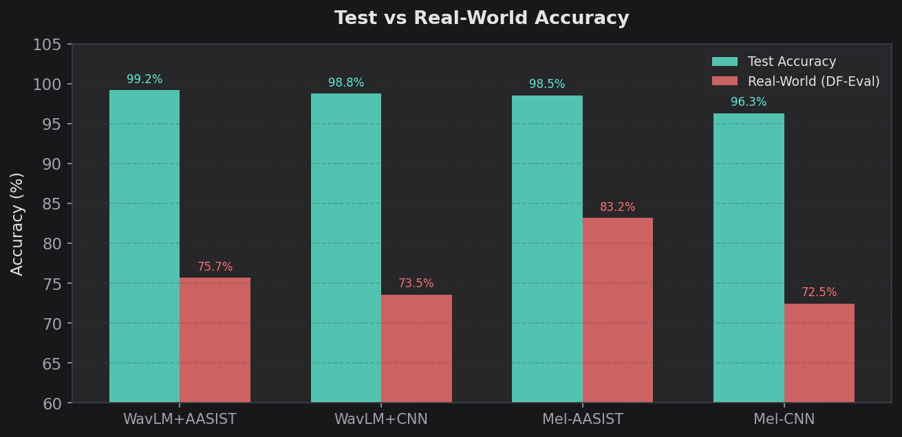
Held-Out Test Set Results (Best Epoch)
| Model | Epochs | Test Acc | Test F1 | Test Prec | Test Recall | Test MCC | Test EER |
|---|---|---|---|---|---|---|---|
| WavLM + AASIST | 15 | 99.18% | 99.25% | – | – | – | 0.0078 |
| WavLM + CNN | 15 | 98.76% | – | – | – | – | 0.0124 |
| Mel-AASIST | 50 | 98.55% | 98.68% | 97.93% | 99.43% | 0.9710 | 0.0121 |
| Mel-CNN | 50 | 96.33% | 96.65% | 95.47% | 97.87% | 0.9262 | 0.0342 |
The ranking made intuitive sense. WavLM + AASIST had the most parameters and the richest features. Mel-CNN had the least. The spread was tight — only 2.85 percentage points separated the best from the worst.
Then I ran Deepfake-Eval-2024.
Deepfake-Eval-2024 Results (Out-of-Distribution)
| Model | Acc | Prec | Recall | F1 | MCC | EER |
|---|---|---|---|---|---|---|
| Mel-AASIST | 83.17% | 78.92% | 80.67% | 0.7978 | 0.6539 | 0.1759 |
| WavLM + AASIST | 75.67% | 84.58% | 50.00% | 0.6285 | 0.5004 | 0.2494 |
| WavLM + CNN | 73.54% | 65.90% | 74.01% | 0.6972 | 0.4662 | 0.2644 |
| Mel-CNN | 72.48% | 62.47% | 83.00% | 0.7129 | 0.4757 | 0.2558 |
The ranking completely inverted. The model that was worst on the test set (by EER) was now best by a wide margin. Mel-AASIST beat the nearest WavLM model by 7.5 percentage points on accuracy and achieved an EER nearly 8 points lower.
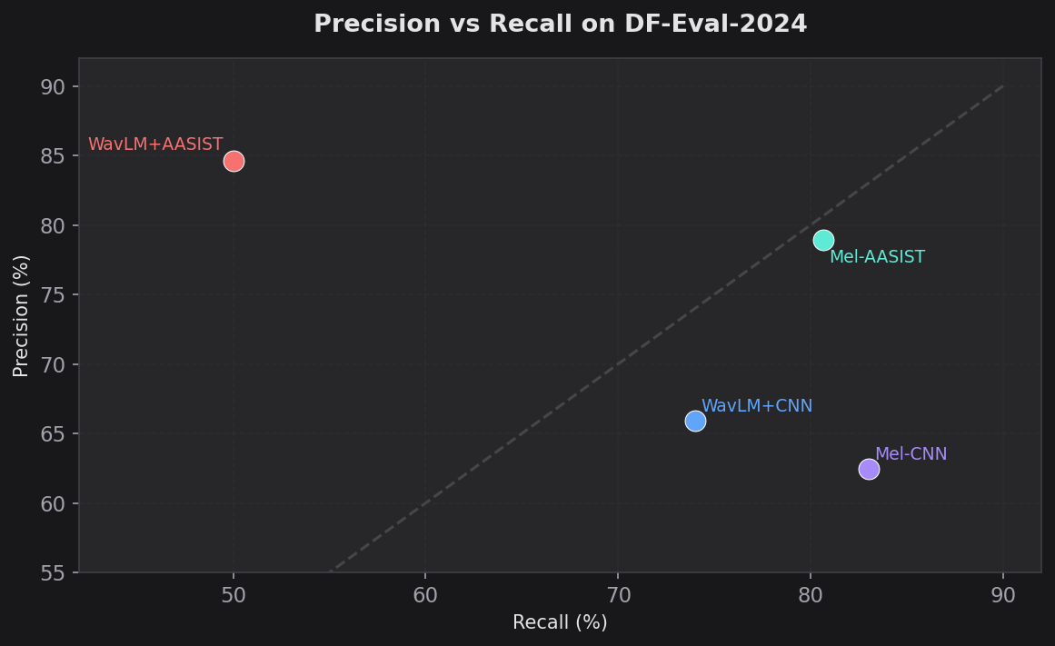
But the precision/recall breakdown reveals something even more interesting about how each model fails:
- WavLM + AASIST had the highest precision (84.58%) but the lowest recall (50.00%). It was conservative — when it flagged something as fake, it was usually right. But it missed half of all deepfakes entirely. A coin flip on whether it catches a fake.
- Mel-CNN had the opposite problem: low precision (62.47%) but high recall (83.00%). It caught most fakes but generated a lot of false positives.
- Mel-AASIST hit the sweet spot: 78.92% precision and 80.67% recall. Balanced performance, which is why its F1 (0.7978) was far ahead of the pack.
- WavLM + CNN landed in the middle on both axes (65.90% precision, 74.01% recall).
The MCC scores tell the same story more starkly. Mel-AASIST at 0.6539 indicates strong agreement between predictions and ground truth. WavLM + CNN at 0.4662 is moderate at best.
Part 2: Training Dynamics
Raw final numbers hide important patterns. Here's how each model evolved during training.
WavLM + CNN Training Curve (15 epochs)
| Epoch | Val Acc | Val EER | Test Acc | Test EER |
|---|---|---|---|---|
| 1 | 87.90% | 0.1210 | 94.38% | 0.0537 |
| 4 | 91.37% | 0.0864 | 97.28% | 0.0291 |
| 10 | 92.32% | 0.0768 | 98.76% | 0.0124 |
| 15 | 91.76% | 0.0824 | 98.63% | 0.0137 |
Notice the val accuracy peaked at epoch 10 (92.32%) and started declining by epoch 15 (91.76%), while test accuracy barely moved. Classic early signs of overfitting. The model squeezed out the last 0.13% of test accuracy between epoch 10 and 15 but lost 0.56% on validation. I should have stopped at epoch 10.
WavLM + AASIST Training Curve (15 epochs)
| Epoch | Val Acc | Val EER | Test Acc | Test F1 | Test EER |
|---|---|---|---|---|---|
| 2 | 89.46% | 0.1054 | 97.40% | 97.60% | 0.0245 |
| 7 | 93.25% | 0.0675 | 99.13% | 99.20% | 0.0090 |
| 11 | 93.19% | 0.0681 | 99.23% | 99.29% | 0.0073 |
| 14 | 93.57% | 0.0643 | 99.18% | 99.25% | 0.0060 |
| 15 | 93.94% | 0.0606 | 99.18% | 99.25% | 0.0078 |
This model trained more stably. Validation EER steadily improved from 0.1054 to 0.0606 over 15 epochs. The test EER peaked at epoch 14 (0.0060) and slightly regressed at epoch 15 (0.0078). The AASIST architecture's attention mechanisms likely helped regularize the frozen WavLM features.
Mel-AASIST and Mel-CNN (50 epochs)
The mel-only models told a different story. The Mel-AASIST reached best validation loss at epoch 14 (val_loss=0.2895), while Mel-CNN hit best validation at epoch 19 (val_loss=0.3454). But — and this is crucial — their Deepfake-Eval performance continued improving well past the point where training loss had converged and validation loss had plateaued.
For Mel-AASIST:
- Train loss at epoch 50: 0.0169 (essentially converged by epoch ~15)
- Final val accuracy: 89.38%, val EER: 0.1062
- But DF-Eval accuracy at epoch 50: 83.17% — a number I never would have reached if I'd stopped at the "optimal" early stopping point
For Mel-CNN:
- Train loss at epoch 50: 0.0992 (higher than AASIST, suggesting the simpler architecture struggled more with the training distribution)
- Final val accuracy: 85.91%, val EER: 0.1409
- DF-Eval accuracy at epoch 50: 72.48%
The gap between validation EER (0.1062 for AASIST vs 0.1409 for CNN) predicted the gap in generalization performance (83.17% vs 72.48% on DF-Eval). Validation EER was a much better predictor of real-world performance than test accuracy.
Part 3: The 100% Accuracy Trap
In a separate set of experiments, I fine-tuned WavLM + AASIST models on my custom dataset instead of ASV5. WavLM stayed frozen. I ran two variants: one trained on clean data, one on corrupted data.
Clean Data Fine-Tuning
| Epoch | Train Loss | Train Acc | Val Acc | Val EER | Test Acc | Test F1 | Test MCC | Test EER |
|---|---|---|---|---|---|---|---|---|
| 1 | 0.0340 | 98.93% | 45.64% | 0.5436 | 95.71% | 97.66% | 0.7542 | 0.0000 |
| 6 | 0.0018 | 99.94% | 46.84% | 0.5368 | 99.92% | 99.96% | 0.9960 | 0.0000 |
| 10 | 0.0006 | 99.98% | 49.68% | 0.5058 | 100.00% | 100.00% | 1.0000 | 0.0000 |
| 15 | 0.0003 | 99.99% | 49.76% | 0.4998 | 100.00% | 100.00% | 1.0000 | 0.0000 |
| 20 | 0.0001 | 100.00% | 50.05% | 0.4980 | 100.00% | 100.00% | 1.0000 | 0.0000 |
Deepfake-Eval (epoch 10): Acc=59.15%, Prec=100.00%, Recall=0.74%, F1=0.0147, MCC=0.0660, EER=0.4870 Deepfake-Eval (epoch 20): Acc=59.25%, Prec=100.00%, Recall=0.99%, F1=0.0195, MCC=0.0763, EER=0.4838
Read those DF-Eval numbers carefully. 100% precision but 0.74% recall. The model almost never predicted "fake" on out-of-distribution data. When it did (7 out of ~810 fake samples), it happened to be right. But it missed 99% of all deepfakes. The 59% accuracy comes almost entirely from correctly labeling real speech as real — because the model learned to call everything real.
The validation set was screaming at me. Val EER hovered at 0.50 from epoch 1 to epoch 20 — literally random chance — while test accuracy climbed to 100%. This is the most extreme train/val divergence I've ever seen. The model didn't learn a single generalizable feature. It memorized every training sample.

Corrupt Data Fine-Tuning
| Epoch | Train Loss | Train Acc | Val Acc | Val EER | Test Acc | Test F1 | Test MCC | Test EER |
|---|---|---|---|---|---|---|---|---|
| 1 | 0.0878 | 96.78% | 43.42% | 0.5658 | 93.69% | 96.59% | 0.6158 | 0.0103 |
| 7 | 0.0145 | 99.48% | 51.05% | 0.4876 | 98.65% | 99.25% | 0.9273 | 0.0041 |
| 14 | 0.0056 | 99.80% | 51.96% | 0.4849 | 98.99% | 99.44% | 0.9460 | 0.0027 |
| 20 | 0.0044 | 99.85% | 50.80% | 0.4960 | 99.23% | 99.57% | 0.9591 | 0.0011 |
Deepfake-Eval (epoch 10): Acc=59.15%, Prec=65.00%, Recall=1.60%, F1=0.0312, MCC=0.0490, EER=0.4931 Deepfake-Eval (epoch 20): Acc=59.00%, Prec=63.64%, Recall=0.86%, F1=0.0170, MCC=0.0342, EER=0.4850
The corrupt variant was slightly less extreme — it didn't hit 100% test accuracy, settling at 99.23%. But the DF-Eval story was identical: ~59% accuracy, sub-1% recall, EER around 0.49. Training on corrupted audio added no regularization benefit whatsoever.
Both models were confidently, perfectly wrong. They solved the training set and learned nothing about deepfakes.
Part 4: The 20-Epoch vs 50-Epoch Story
One of my most actionable findings came from comparing the same architecture at different training lengths.
I ran Mel-AASIST for 20 epochs on clean ASV5 FLAC in the ablation study, and separately for 50 epochs on the ASV5 balanced dataset.
Mel-AASIST at 20 Epochs (ASV5 FLAC Clean)
| Epoch | Train Loss | Train Acc | Val Acc | Val EER | Test Acc | Test F1 | Test EER |
|---|---|---|---|---|---|---|---|
| 1 | 0.1086 | 96.20% | 67.60% | 0.3238 | 97.19% | 98.45% | 0.0382 |
| 8 | 0.0041 | 99.88% | 66.13% | 0.3386 | 98.21% | 99.01% | 0.0010 |
| 12 | 0.0028 | 99.91% | 66.59% | 0.3340 | 98.74% | 99.30% | 0.0010 |
| 15 | 0.0014 | 99.96% | 66.22% | 0.3377 | 98.53% | 99.18% | 0.0010 |
| 20 | 0.0006 | 99.98% | 64.73% | 0.3526 | 98.05% | 98.92% | 0.0041 |
DF-Eval (epoch 10): Acc=59.96%, Prec=54.58%, Recall=16.13%, F1=0.2490, MCC=0.1015, EER=0.4763 DF-Eval (epoch 20): Acc=58.59%, Prec=47.97%, Recall=7.27%, F1=0.1262, MCC=0.0357, EER=0.5161
At 20 epochs: 58.59% DF-Eval accuracy, 0.5161 EER. Essentially random.
Mel-AASIST at 50 Epochs (ASV5 Balanced)
At 50 epochs: 83.17% DF-Eval accuracy, 0.1759 EER.
That's a 24.6 percentage point jump in DF-Eval accuracy and a 0.34 drop in EER just from training longer. The training loss was already near zero by epoch 15 in both runs. By conventional early stopping logic, there was no reason to keep training. But the model was still learning something — some slow-forming, generalizable representation of what makes audio fake — that only showed up on out-of-distribution data.
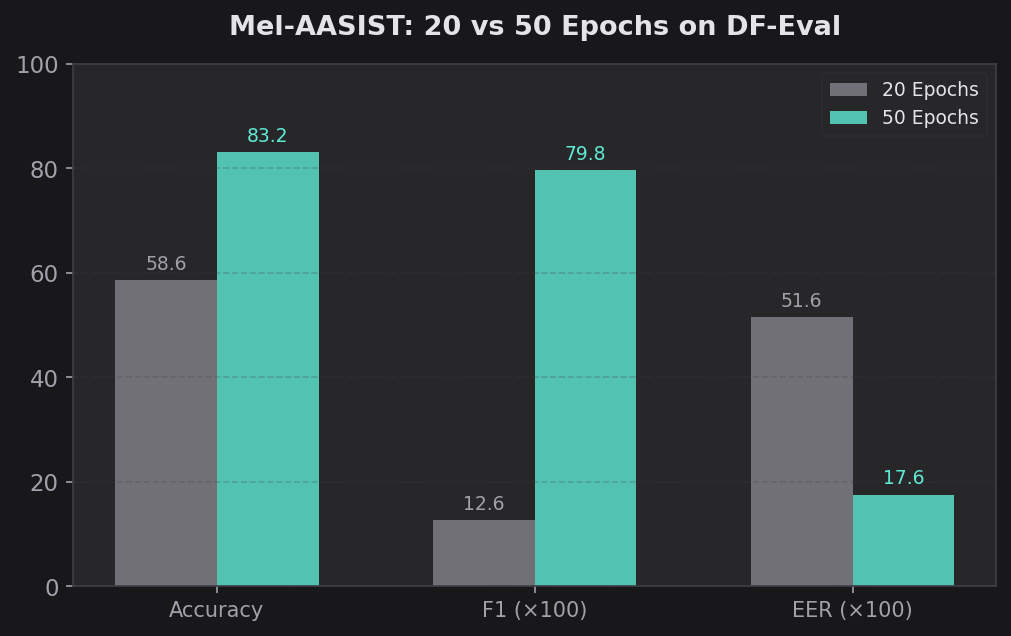
This has significant practical implications. If you're training a deepfake detector and evaluating only on in-distribution metrics, you'll stop too early. The features that generalize take longer to learn than the features that memorize.
Two additional observations from the 20-epoch run:
- Validation EER was around 0.33 throughout — much better than the ~0.50 seen in the WavLM fine-tuning experiments. The mel-only model was at least learning some transferable features, even at 20 epochs.
- Test accuracy actually degraded slightly from epoch 12 (98.74%) to epoch 20 (98.05%), suggesting the model was beginning to overfit to training data, yet DF-Eval could have improved with more training. In-distribution and out-of-distribution performance can move in opposite directions.
Part 5: The Codec and Data Ablation
I ran a systematic ablation across audio formats, data corruption, and training data source. Six CNN variants were trained and evaluated on Deepfake-Eval-2024 at a decision threshold of 0.5:
| Variant | Dataset | Format | Corrupt | Acc | Prec | Recall | F1 | MCC | Spec |
|---|---|---|---|---|---|---|---|---|---|
| Clean Custom CNN | Custom | Mixed | No | 77.33% | 87.18% | 52.47% | 0.6551 | 0.5372 | 94.63% |
| Corrupt Custom CNN | Custom | Mixed | Yes | 75.93% | 89.64% | 46.76% | 0.6146 | 0.5157 | 96.24% |
| FLAC CNN | ASV5 | FLAC | No | 61.56% | 79.71% | 8.49% | 0.1534 | 0.1681 | 98.50% |
| FLAC Corrupt CNN | ASV5 | FLAC | Yes | 53.39% | 32.81% | 12.96% | 0.1858 | -0.0736 | 81.53% |
| MP3 CNN | ASV5 | MP3 | No | 59.78% | 65.12% | 4.32% | 0.0810 | 0.0819 | 98.39% |
| MP3 Corrupt CNN | ASV5 | MP3 | Yes | 41.04% | 41.04% | 100.00% | 0.5819 | 0.0000 | 0.00% |
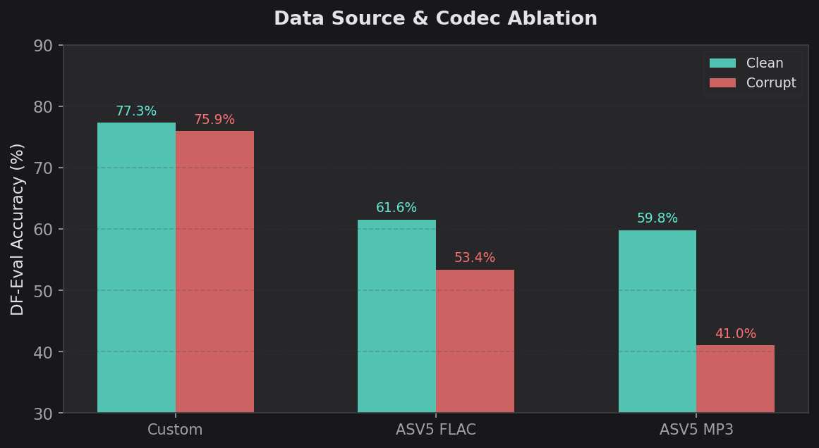
There are several stories in this table:
1. Data source dominates everything. Custom dataset models (77.33%, 75.93%) crushed ASV5 models (41-62%) regardless of codec or corruption. The custom dataset included samples from more deepfake generators, and that diversity was the single largest lever for generalization. A 15-18 percentage point gap from data diversity alone.
2. Codec matters, but less than data source. Within ASV5, FLAC (61.56%) slightly outperformed MP3 (59.78%) on clean data. FLAC preserves more spectral detail that the model can use to distinguish real from fake. MP3 compression smears the very artifacts the detector needs to find.
3. Corruption is neutral to harmful. Clean vs corrupt performance within the same data source:
- Custom: 77.33% clean vs 75.93% corrupt (-1.4%)
- ASV5 FLAC: 61.56% clean vs 53.39% corrupt (-8.2%)
- ASV5 MP3: 59.78% clean vs 41.04% corrupt (-18.7%)
Corruption never helped. On ASV5 MP3, it was catastrophic — the corrupt model collapsed to 41% accuracy with 0.00% specificity, meaning it classified every single sample as fake.
4. Failure modes differ dramatically. The FLAC and MP3 CNN models were extremely conservative (very high specificity of 98%+, very low recall of 4-13%). They almost never flagged anything as fake. The MP3 corrupt model went the other direction entirely — 100% recall, 0% specificity, labeling everything as fake. The custom dataset models landed in a healthier middle ground.
5. The MCC reveals the true picture. The FLAC corrupt CNN had a negative MCC (-0.0736), meaning its predictions were anti-correlated with ground truth. It would have been more accurate if you flipped its labels. The MP3 corrupt CNN had MCC of exactly 0.0000 — no correlation at all, identical to random guessing (which makes sense given its predict-everything-as-fake strategy).
I also ran AASIST variants in the same ablation across ASV5 FLAC and MP3, plus a standalone ablation of Mel-AASIST on the custom dataset. The numbered result directories (01-12) capture the full matrix:
| # | Config | Arch | Data | Corrupt |
|---|---|---|---|---|
| 01 | Custom AASIST + WavLM | AASIST | Custom | Clean |
| 02 | Custom AASIST + WavLM | AASIST | Custom | Corrupt |
| 03 | Custom CNN + WavLM | CNN | Custom | Clean |
| 04 | Custom CNN + WavLM | CNN | Custom | Corrupt |
| 05 | ASV FLAC AASIST Mel | AASIST | ASV5 FLAC | Clean |
| 06 | ASV FLAC AASIST Mel | AASIST | ASV5 FLAC | Corrupt |
| 07 | ASV FLAC CNN Mel | CNN | ASV5 FLAC | Clean |
| 08 | ASV FLAC CNN Mel | CNN | ASV5 FLAC | Corrupt |
| 09 | ASV MP3 AASIST Mel | AASIST | ASV5 MP3 | Clean |
| 10 | ASV MP3 AASIST Mel | AASIST | ASV5 MP3 | Corrupt |
| 11 | ASV MP3 CNN Mel | CNN | ASV5 MP3 | Clean |
| 12 | ASV MP3 CNN Mel | CNN | ASV5 MP3 | Corrupt |
Plus cross-domain transfer experiments fine-tuning ASV5-pretrained WavLM+AASIST models on the custom holdout set (clean and corrupt variants, three runs each with different timestamps).
Part 6: Earlier Experiments and the Polished vs Unpolished Gap
Before the systematic ablation, I ran earlier WavLM + CNN experiments that revealed another important finding: the gap between "polished" and "unpolished" evaluation data.
These earlier runs used two validation sets simultaneously — an unpolished holdout (raw recordings) and a polished holdout (cleaned/curated recordings):
| Run | Epochs | Val Acc (Unpol.) | Val EER (Unpol.) | Val Acc (Pol.) | Val EER (Pol.) | Test Acc |
|---|---|---|---|---|---|---|
| Resumed ep. 17 | 18 | 93.22% | 0.0677 | 86.32% | 0.1377 | 97.77% |
| Resumed ep. 17 | 19 | 92.48% | 0.0752 | 86.73% | 0.1347 | – |
| Fresh start | 1 | 91.93% | 0.0807 | 85.16% | 0.1537 | 92.81% |
| Large dataset | 1 | 84.29% | 0.1570 | 81.04% | 0.1498 | 98.46% |
The polished data was consistently harder — a 5-7 percentage point accuracy gap and roughly double the EER. This is important because real-world deepfakes are increasingly polished. A detector that works on raw generator output but fails on post-processed audio has limited practical value.
The large dataset run is also notable: despite only reaching 84.29% validation accuracy after 1 epoch, it hit 98.46% test accuracy. This suggests the model was rapidly memorizing the test distribution while struggling with the validation set's diversity — another early signal of the overfitting pattern I'd see more dramatically in later experiments.
Part 7: Why Did the Small Model Win?
I don't have a definitive answer, but the data points toward a hypothesis.
The WavLM representation space is too specific. WavLM was pretrained to understand speech — phonemes, prosody, speaker identity, linguistic content. When you freeze those representations and train a binary classifier on top, the classifier learns to detect artifacts in the space of speech representations. Those artifacts turn out to be specific to whatever deepfake generators exist in the training data. When the generator changes, the artifacts in WavLM-space change too, and the classifier breaks.
The evidence for this: WavLM models achieved the highest test accuracy (99.18%) but showed the most dramatic DF-Eval degradation. The frozen features are powerful enough to perfectly separate training-distribution real from fake, but that separation doesn't generalize.
Mel-spectrograms force more universal feature learning. Mel-AASIST operates directly on mel-spectrograms. It has to learn its own features from scratch. With multi-scale convolutions (3x3, 5x5, and dilated 7x7 kernels), it's forced to find patterns at multiple time-frequency resolutions simultaneously. Squeeze-and-excitation attention lets it learn which frequency bands matter most. Attentive statistics pooling lets it learn which time frames are most informative.
These patterns — subtle spectral inconsistencies, unnatural harmonic structures, phase artifacts, overly smooth formant transitions — appear to be more universal across different deepfake generators than whatever the WavLM classifier was latching onto.
The parameter count constraint may be a feature, not a bug. With only ~2M parameters (vs 350M+), Mel-AASIST can't memorize as easily. It's forced into compression — finding compact, generalizable representations rather than storing specific examples. This is the classic bias-variance tradeoff manifesting in a particularly dramatic way.
The recall pattern supports this. WavLM + AASIST achieved 84.58% precision but only 50% recall on DF-Eval. It was confident when it predicted "fake" but missed half of all fakes. This suggests it learned a narrow set of generator-specific tells — when it saw those tells, it was right, but most out-of-distribution fakes don't have those specific tells. Mel-AASIST achieved 78.92% precision and 80.67% recall — a more balanced detector that recognizes a wider variety of fakeness signals.
The Complete Picture
Putting all results together in one table, ranked by Deepfake-Eval accuracy:
| Rank | Model | Data | Ep | Test Acc | DF-Eval Acc | DF-Eval F1 | DF-Eval EER |
|---|---|---|---|---|---|---|---|
| 1 | Mel-AASIST | ASV5 bal. | 50 | 98.55% | 83.17% | 0.7978 | 0.1759 |
| 2 | Clean Custom CNN | Custom | 3 | – | 77.33% | 0.6551 | – |
| 3 | Corrupt Custom CNN | Custom | 10 | – | 75.93% | 0.6146 | – |
| 4 | WavLM + AASIST | ASV5 | 15 | 99.18% | 75.67% | 0.6285 | 0.2494 |
| 5 | WavLM + CNN | ASV5 | 15 | 98.76% | 73.54% | 0.6972 | 0.2644 |
| 6 | Mel-CNN | ASV5 bal. | 50 | 96.33% | 72.48% | 0.7129 | 0.2558 |
| 7 | FLAC CNN | ASV5 FLAC | 3 | – | 61.56% | 0.1534 | – |
| 8 | Mel-AASIST | ASV5 FLAC | 20 | 98.05% | 58.59% | 0.1262 | 0.5161 |
| 9 | MP3 CNN | ASV5 MP3 | 1 | – | 59.78% | 0.0810 | – |
| 10 | WavLM+AASIST (FT clean) | Custom | 20 | 100.00% | 59.25% | 0.0195 | 0.4838 |
| 11 | WavLM+AASIST (FT corr.) | Custom | 20 | 99.23% | 59.00% | 0.0170 | 0.4850 |
| 12 | FLAC Corrupt CNN | ASV5 FLAC | 2 | – | 53.39% | 0.1858 | – |
| 13 | MP3 Corrupt CNN | ASV5 MP3 | 9 | – | 41.04% | 0.5819 | – |
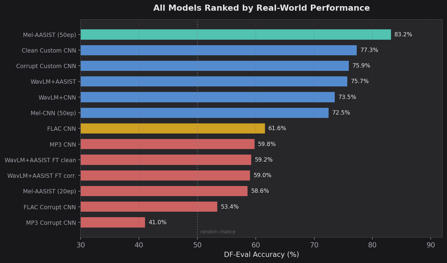
The correlation between test accuracy and DF-Eval accuracy is essentially zero. The model with the highest test accuracy (100.00%) had one of the worst DF-Eval scores (59.25%). The model with the lowest test accuracy in the main comparison (96.33%) outperformed two of the three WavLM models on DF-Eval.
Lessons Learned
1. Test set accuracy is nearly meaningless for deepfake detection. Every main model scored above 96% on held-out test data. The gap between the best and worst on real-world data was over 24 percentage points. The correlation between the two was negative. If you're evaluating a deepfake detector and only reporting in-distribution accuracy, you're not measuring anything useful.
2. Bigger models aren't better — they're better at memorizing. WavLM-Large has 175x more parameters than Mel-AASIST. Those extra parameters bought better memorization of the training distribution and worse generalization to everything else. The frozen SSL features, which are supposed to provide "general" audio understanding, actually created a representation space where overfitting was easier, not harder.
3. Perfect scores are a red flag, not a celebration. When your model hits 100% accuracy, your first reaction should be suspicion, not satisfaction. In my case, 100% test accuracy coexisted with coin-flip performance on real-world data. The model hadn't solved deepfake detection. It had solved the training set.
4. Data diversity beats data quantity, model size, and architecture. The single biggest lever for Deepfake-Eval performance wasn't architecture or parameter count — it was training on data from diverse deepfake generators. A 400K parameter CNN trained on my custom dataset (77.33%) outperformed a 350M+ parameter WavLM model trained on ASV5 (73.54%). The custom dataset models outperformed ASV5 models by 15-18 percentage points across the board.
5. Train longer than you think you need to. Mel-AASIST went from 58.59% DF-Eval accuracy at 20 epochs to 83.17% at 50 epochs. Training loss had converged by epoch 15. The generalizable features took 3x longer to form than the memorization features. Conventional early stopping based on validation loss would have killed the run before the good features emerged.
6. Audio codec choice matters. FLAC-trained models consistently outperformed MP3-trained models. MP3 compression destroys the subtle spectral artifacts that differentiate real from fake audio. If you're building a deepfake detector, train on lossless audio.
7. Data corruption doesn't help. Clean vs corrupt training showed negligible differences at best and catastrophic degradation at worst (MP3 corrupt: 41% accuracy). The bottleneck is exposure to diverse generation methods, not robustness to noise. Don't waste cycles on audio corruption augmentation for this task.
8. Watch your validation set, not your test set. In the WavLM fine-tuning experiments, validation accuracy sat at ~50% while test accuracy climbed to 100%. That 50-point divergence was the model screaming that it was overfitting. In the mel-only experiments, validation EER (0.10 for AASIST vs 0.14 for CNN) correctly predicted which model would generalize better. The validation set is your early warning system — trust it over the test set.
9. Precision/recall balance predicts real-world utility. High precision with low recall (WavLM + AASIST: 84.58% / 50.00%) means the model is conservative but misses most fakes. High recall with low precision (Mel-CNN: 62.47% / 83.00%) means it catches fakes but generates false alarms. Balanced precision and recall (Mel-AASIST: 78.92% / 80.67%) is what you want for a production system. Accuracy alone doesn't tell you this.
10. The polished data gap is real. Earlier experiments showed a consistent 5-7 percentage point accuracy drop when evaluating on polished (post-processed) audio vs raw audio. Real-world deepfakes are increasingly polished. Evaluation on raw generator output overestimates real-world performance.
Model Size vs Performance
| Architecture | Params | Size | DF-Eval Acc | DF-Eval EER | Acc/MB |
|---|---|---|---|---|---|
| Mel-CNN | ~400K | 435 KB | 72.48% | 0.2558 | 166.6%/MB |
| Mel-AASIST | ~2M | 2.2 MB | 83.17% | 0.1759 | 37.8%/MB |
| WavLM + CNN | ~350M | ~1.3 GB | 73.54% | 0.2644 | 0.06%/MB |
| WavLM + AASIST | ~350M | ~1.3 GB | 75.67% | 0.2494 | 0.06%/MB |
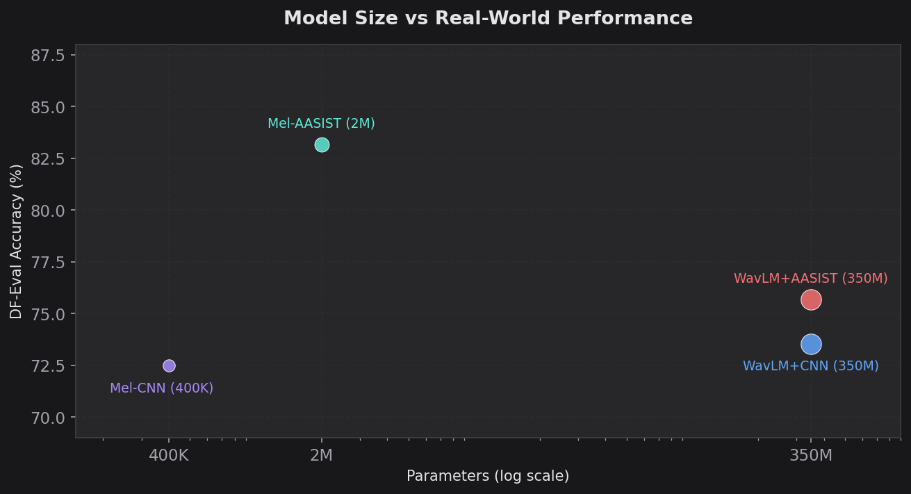
Mel-AASIST delivers the best absolute performance at 2.2 MB. The WavLM models are 590x larger for worse results. Mel-CNN is the efficiency champion on a per-megabyte basis but trails on absolute performance.
For production deployment where model size, latency, and compute cost matter, Mel-AASIST is the clear winner by every metric.
The uncomfortable truth about audio deepfake detection is that the field has a generalization problem. Models that look incredible on benchmarks fall apart when the generator changes. My results suggest that the path forward isn't bigger pretrained models — it's architectures and training strategies that force the model to learn universal artifacts rather than generator-specific fingerprints.
Sometimes less really is more.